Extracting Geomorphic Covariance Structure (GCS) series

In this step we extract width (W) and mean detrended bed elevation (Z), a inverse proxy for depth, across the longitudinal extent of the river segment via dense, evenly spaced, cross-sectional rectangles (see examples). W and Z value are standardized to capture relative cross-sectional geometry, yielding Ws and Zs respectively. Cross-sections with Ws > 0 are wider than the mean, and cross-sections with Zs > 0 are shallower (higher bed elevation) than the mean. Multiplying Ws and Zs, due to the their standardized nature (see interpreting results) calculates their covariance at a given cross section, C(Ws, Zs). Each cross-sections W, Z, Ws, Zs, C(Ws, Zs) value are stored in a csv file that is the basis for Geomorphic Covariance Structure analysis (see Literature).

Inputs

• The detrended DEM, ras_detren.tif

• Key flow stage elevations separated by commas, ex: ‘0.2,0.7,2.6’

• USER INPUT: Cross-section spacing in the same units as the DEM

  • Spacing should be >= DEM resolution.

  • Typically defined relative to river width. Past analysis used 1/20th of typical bankfull width.

• USER INPUT: Cross-section lengths for each key flow stage separated by commas, ex: ‘200,400,1000’

  • In the same units as the DEM

  • Must be entered corresponding to the key flow stage elevation order. ex: ‘0.2,0.7,2.6’ / ‘200,400,1000’ where 200m cross-sections are used for the 0.2m flow stage.

  Important

  Please see the choosing cross-section lengths section below before defining cross-section lengths!

Extracted cross-sectional values

• Values represents the mean of a given cross-sectional polygon, which has a length set by the cross-section spacing parameter.

• A new folder, gcs_tables/ is made to store .csv files with all cross-sectional data for each flow stage, ex: gcs_tables/0p2m_gcs_table.csv

Extracted values and their .csv file headers:

• Width : W

• Detrended bed elevation : Z

• Mean elevation : elevation (not detrended)

• Mean depth : d_mean = flow stage height - Z

• Width / depth ratio : wd_ratio

• Standardized width : Ws = cross-section W - river mean W / river W standard deviation

• Standardized detrended bed elevation : Zs = cross-section Z - river mean Z / river Z standard deviation

• Ws, Zs covariance, C(Ws, Zs) : Ws_Zs = Ws * Zs

Choosing cross-section lengths

The user must define the desired cross-section length for each key flow stage.

There are two ways for defined cross-section lengths to generate erronous results:

1. The cross-sections are not long enough to extend accross the wetted area of a given flow stage. This results in truncated cross-section width values.

   • In the example below, 20ft cross-secctions were created for a 0.2ft flow stage. As you can see, some fail to extend across the wetted area.

   

2. The cross-sections are too long relative to the centerline sinuousity, and re-cross the wetted area polygon’s perimeter at multiple locations. Or are long enough to intersect discconected topographic lows.

   • Either cross-section re-crossing or coverage of isolated topographic lows can result in erronous width values.

   • An example with both issues is below. 500ft cross-sections are shown for a 0.2ft flow stage.

   

Tip

Try to find the widest segment of each flow stage wetted area polygon. Use the ruler tool in ArcPro or ArcMap to measure the distance from the centerline to the wetted polygon perimeter at an estimated width maxima. Doubling that distance (and adding to that sum slightly) is a good way to establish a minimum cross-section length for each flow stage.

Most rivers become less sinuous as flow stage increases. Therefore a cross-secction length long enough to cover the highest key flow stage is likely to cause re-crossing when applied to lower, more sinuous flow stages. For some very straight rivers a single cross-section length may suit all flow stages, but still must be input separately (i.e. ‘500,500,500,500’).

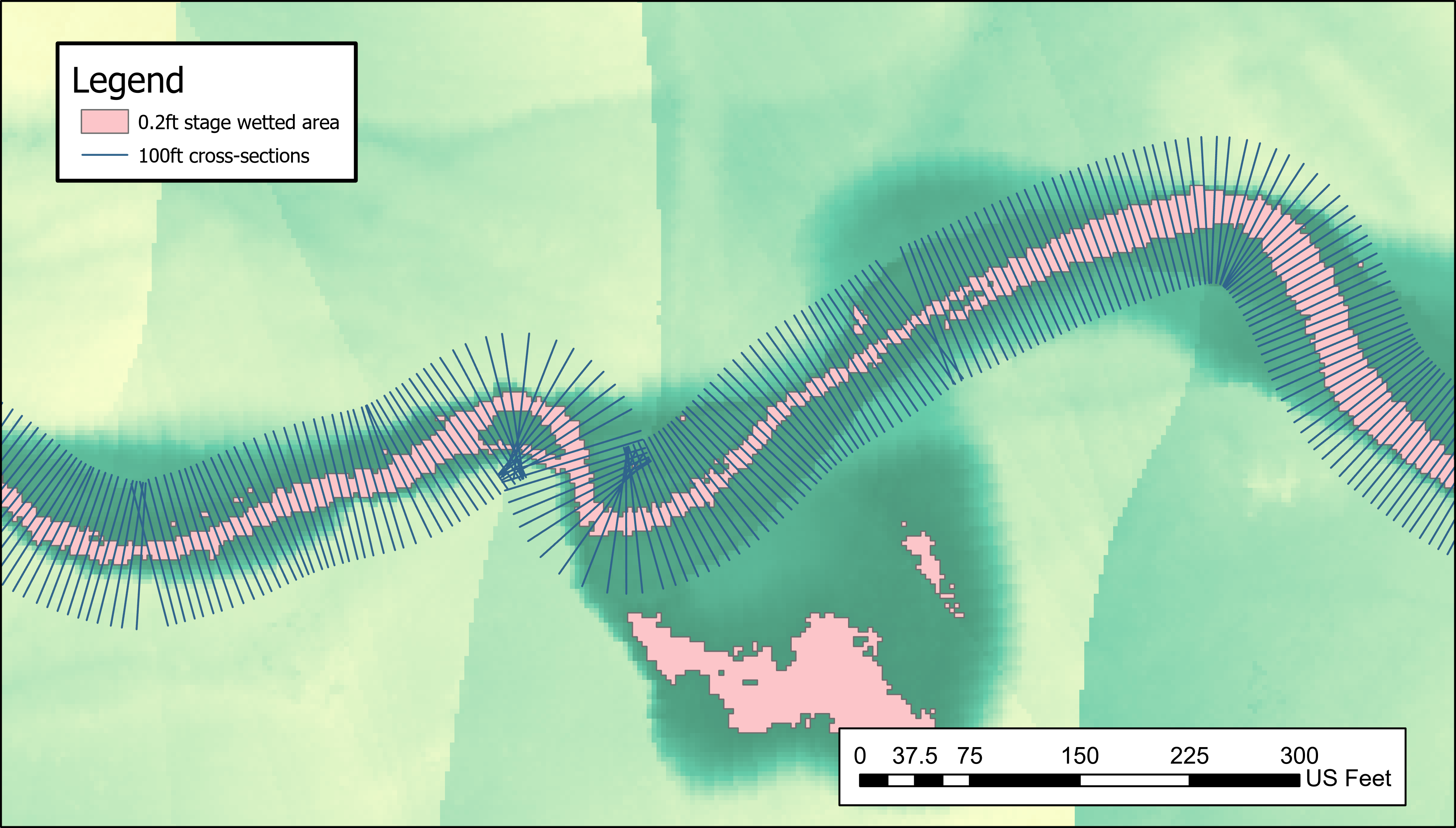
Finally, below we see an example of an appropriately selected cross-section length for the 0.2ft flow stage.

Using a clip polygon (optional)

There is the option to further reduce / clip the study area before extracting GCS series. This is done by manually generating a polygon that overlaps with what should be included and defining it’s spatial reference to match the project.

We generally use clip polygons for one of two reasons:

1. To reduce the longitudinal extent of the study area.

2. To exclude wetted area polygon quality issues related to DEM detrending artefacts.

For example, we can see below that there low lying areas of the floodplain are erroneously included in the 2.6 ft flow stage wetted area polygon. Here we made the clip polygon (black) that to excludes such errors, resulting in the quality cross-section polygons shown in the figure.

Another strategy is altering cross-section lengths, which can work in most settings where the issues are far from the channel.

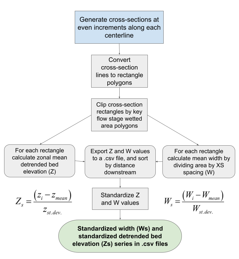
Applied method flow chart